Multi Channel Analyzer (MCA)
The digital multi-channel analyzer allows the estimation of the energy spectrum from a nuclear radiation detector using various digital signal processing methods. All methods work in real time independently for each channel without the need to reprogram the device.
Multi Channel Analyzer Tab
The MCA tab contains two charts. The waveforms displayed in the left graph are mostly debug time domain waveforms and are decimated by 4. It is possible to display two different waveforms at the same time. The source of the displayed signal is selected using the “Debug 1 source” and “Debug 2 source” selectors. The functionality of the right graph is constant and contains a measured energy spectrum containing 16384 energy channels.
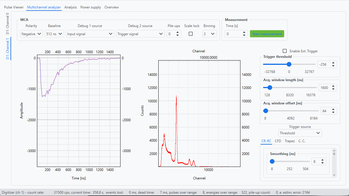
The MCA settings
Polarity
Selector for input signal polarity - “Positive” or “Negative”
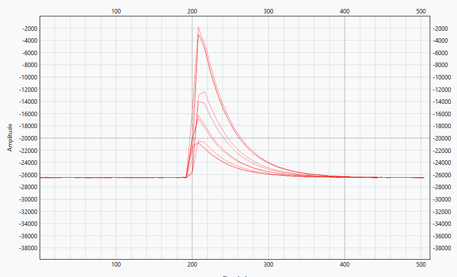
Polarity - Positive
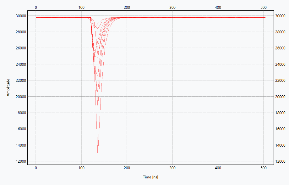
Polarity - Negative
Baseline
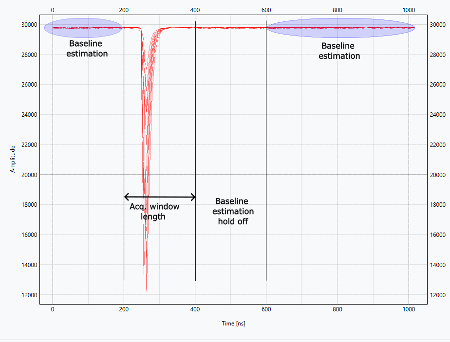
The baseline is a DC level of the signal and should be removed from the pulse (similar to AC coupling) to estimate pulse energy using the pulse charge integration method. The baseline parameter is the moving average filter window length. The baseline level is calculated continuously using a signal between detected pulses. Baseline level calculation is held off when the pulse is detected in Acq. window length and just after the pulse during the same time as Acq. window length.
Note
Baseline moving average filter window length has a direct impact on energy spectra quality. Short filter window length may decrease energy estimation quality and as a consequence increase FWHM.
Debug 1 source
First debug signal visible on left graph:
Input signal
Signal minus estimated baseline. This signal is used for pulse energy estimation using the pulse charge integration method.
Trigger signal
Output signal from active pulse detection module. Threshold detection on input signal or threshold detection on CR-RC filter output.
Trapezoid signal
Trapezoid filter output signal.
Trapezoid energy window
Trapezoid filter energy estymation window.
CFD signal
Constant Fraction Discriminator filter output.
CFD ZC window
Constant Fraction Discriminator zero-crossing detection window.
Charge Comparison
Part of input signal using in Charge Comparison method.
Debug 2 source
Second debug signal visible on left graph. Usage and options are the same as Debug 1 source.
Pile-ups
Any value higher than 0 enables a pile-up detector and sets pile-up events limit in a single acquisition window. When pile-up is detected acquisition window is extended by Acq. Window length to cover all detected pulses.
Note
The pile-up detector is sensitive to signal noise. High noise amplitude on a slow fall signal part may cause false pile-up detection.
Binning
Energy spectrum binning coefficient.
Time
Set measurement time.
Trigger threshold
The value of trigger threshold is referenced to 0 level. Rising edge detector is used for positive pulse and as a consequence falling edge detector is used for negative pulse.
Note
When adjusting the trigger level of a digitizer the user should keep in mind that the digitized samples are represented in a range from -2^Nbit to (2^Nbit - 1) scale (when Nbit is the number of bit of the digitizer ADC) but the digitizer input dynamic range scale is not calibrated and cannot be used as a reference for absolute measurements like a standard oscilloscope but just for relative ones.
Note
When adjusting the trigger level of a digitizer the user should keep in mind that the same threshold level is used in a pile-up detection circuit.
Acq. window length
Acquisition window of the signal used in pulse energy estimation.
Note
A signal acquisition window higher than the pulse duration may have a negative impact on the accuracy of the pulse energy estimate.
Acq. window offset
Acquisition window offset allows you to adjust the signal position relative to the entire acquisition window.
Pulse Shape Discrimination
Pulse shape discrimination allows to distinguish signals originating from different processes for example neutrons and gammas.
To start the PSD measurement first and foremost one has to check the Save streaming option in Options -> Data streaming settings while an MCA tab is active.
Then in the C. C. (Charge comparison) settings tab check Enable Charge Comparison.
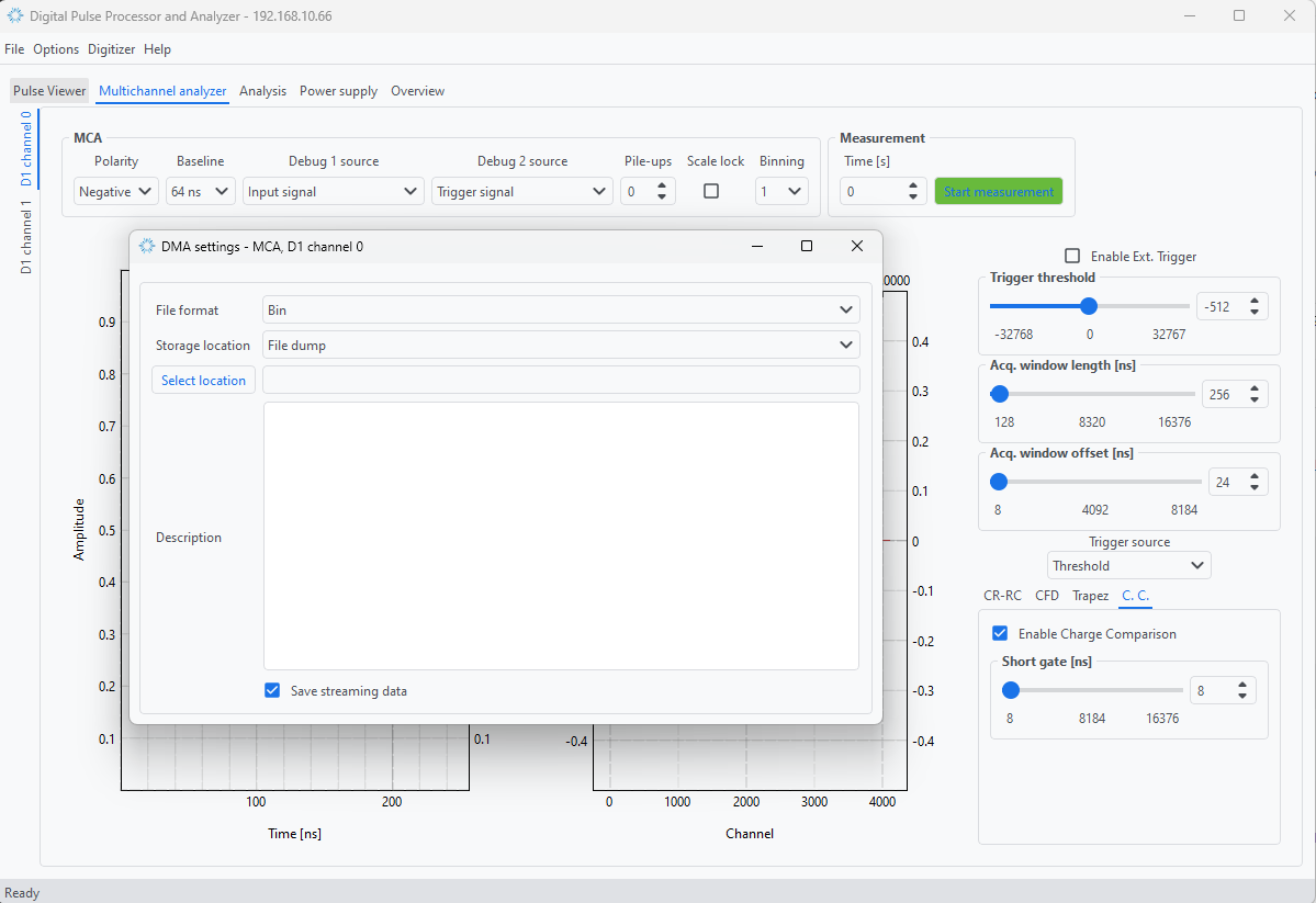
Next step is to properly select the Short gate length. After toggling the measurment, the gated impulse can be monitored by selecting CC gate from Debug 1/2 dropdown lists.
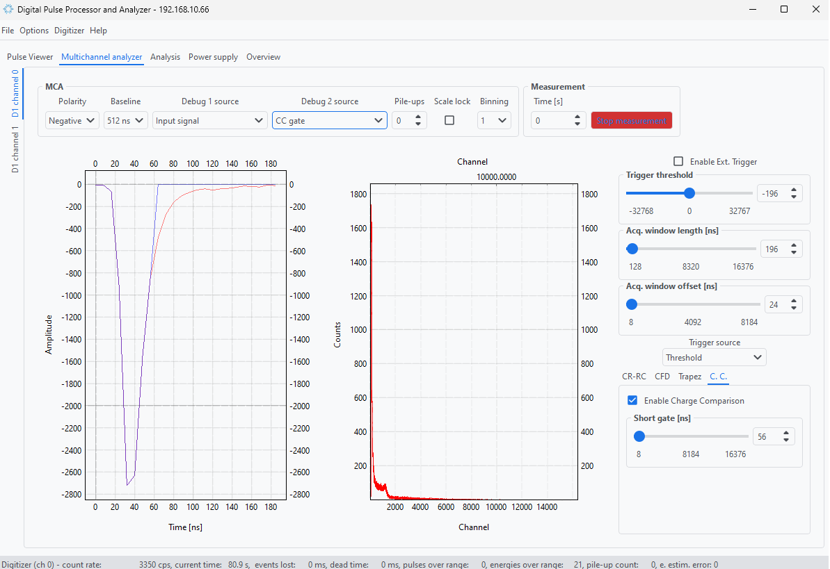
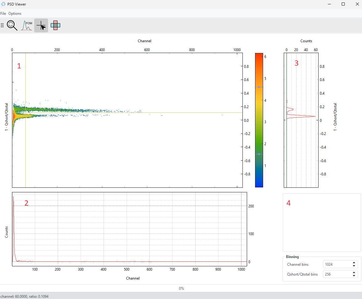
When the measurement is stared a new PSD panel will show up corresponding to the selected channel. The panel cosists of four main areas. Area denoted as 1 presents the 2D histogram of the energies vs ratio of the short impulse integral vs. integral of the whole impulse. The distinct two band shape visible corresponds to two families of events. While moving the coursor over the 1 plot the areas 2 and 3 will update with events corresponding the the bins under the green crosshair lines. The lower plot 2 is a pulse height spectrum and graph 3 is the charge ratio for a given energy.
Note
The values of counts in the PSD histogram (1) were logarithmized to improve visibility of features in the plot.
Note
The crosshair can be dropped by pressing spacebar when the PSD panel is in focus. ctrl and shift can be used to lock x and y axes respectively when zooming the plot with mouse wheel
Note
The scales y of 2 and 3 can be changed to log by pressing ‘l’ key (low-case ‘L’) when the PSD panel is in focus.
Instead of selecting only signle channels with the crosshair the selection can be changed to Regions of Interests for both scales using the Select region of interst button from the toolbar. This way the user can sum all the events in the given ROI to improve the number of counts. Finally, a Figure of Merit that describes the separation factor of the neutrons and gammas can be calculated using the Calculate FOM button on the toolbar.